3152 Lecture 5

Lecture Slide: FIT3152 Lecture 05.pdf

Previous: 3152 Lecture 4 - Regression Modelling Next: 3152 Lecture 6 - Decision Tree

Clustering

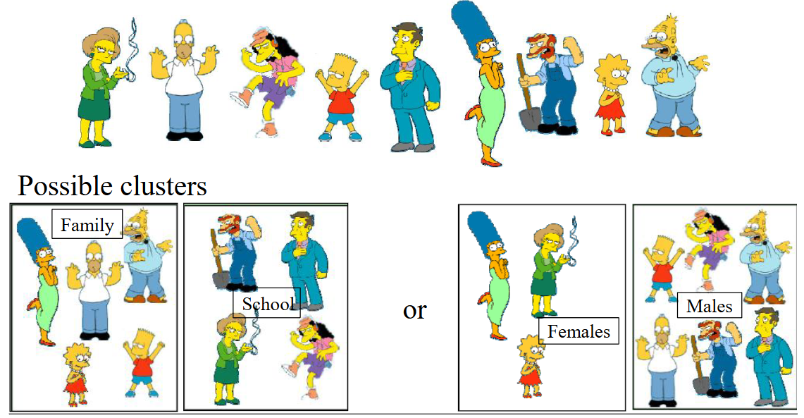
Clustering is unsupervised learning method. The purpose cluster the unlabelled data. Which means it separate the data in to multiple group based on the observed pattern of the data.

Clustering can also be used in real world like group houses based on similar features, clustering the email by content etc.

K-Means Clustering

In K-Means Clustering, each cluster is associated with a centroid (centre point). The rest of points will be assigned to nearest centroid to be come a cluster. Number of cluster $k$ must be specified in order to set the number of centroid.

The K-Means Clustering will do the below process:

1. Randomly select $k$ centroids
2. Assigned each point to nearest centroid to form $k$ clusters
3. Among each cluster, find the new centroid at the centre of cluster
4. Repeat the step of Sign and recompute centroid until centroids doesn’t change or doesn’t change much

Euclidean distance

By using the Euclidean distance we can know how far between two points. It basically use Pythagoras Theorem.

$$\text{Since }c^2=a^2+b^2,\text{therefore } c = \sqrt{(a^2+b^2)}$$

This can also represent as $d(c,x)$, where: $d(x,c)=\sqrt{(x_1-c_1)^2+(x_2-c_2)^2+\cdots+(x_d-c_d)^2}$ Basically, the purpose of K-Means clustering is to minimize the total squared distance of each point to its cluster centroid.

[!NOTE] K-Median K-median will use the total absolute distance rather than squared distance. Squared distance is more aware of outliers, and absolute distance is more robust but harder to find centroid because centroid is likely to have same total absolute distance.

For more information, see Extra Note - K-medians

This could be written as: $\sum_{i=1}^{k}\sum_{j=1}^{n_i} d(c_i,x_{i,j})^2$ Where:

$$\begin{aligned} k &= \text{the number of clusters} \\ c_i &= \text{the centroid of cluster } i,\ i=1,\ldots,k \\ n_i &= \text{the number of points in cluster } i \\ x_{i,j} &= \text{the } j\text{th point of cluster } i \\ d(c_i,x_{i,j}) &= \text{the distance between } c_i \text{ and } x_{i,j} \end{aligned}$$

Evaluate

To evaluate the K-Means clustering, we simply compare the total squared distance above, this is also known as Sum of Squared Error (SSE). By changing the $k$, the SSE changes, we will find the $k$ that has smallest SSE.

However, the easiest way to reduce SSE is to increase $k$, because more clusters usually make points closer to their own centroid.

So SSE should not be used alone.

[!NOTE] SSE This is also mentioned in 2086 Lecture 3 - Estimation and Maximum Likelihood#Sum of the squared error. In FIT2086, we use SSE to minimise the distance between sample values and one estimated mean $\hat{\mu}$.

In K-means, this idea is extended to K means, where each centroid minimises the within-cluster SSE.

$$SSE(c)=\sum_{j=1}^{n} d(c,x_j)^2$$ $$SSE_{total} = \sum_{i=1}^{k}SSE(c_i) = \sum_{i=1}^{k}\sum_{j=1}^{n_i} d(c_i,x_{i,j})^2$$

Silhouette

Silhouette is another method to evaluate clustering.

It measures how well each data point sits within its cluster.

For each point $i$:

$$a_i = \text{average distance from point } i \text{ to other points in the same cluster}$$ $$b_i = \text{smallest average distance from point } i \text{ to points in another cluster}$$

The silhouette score is:

$$s_i=\frac{b_i-a_i}{\max(b_i,a_i)}$$

Ideally, $a_i$ should be small and $b_i$ should be large.

This means the point is close to points in its own cluster, and far from points in other clusters.

The value of $s_i$ is between -1 and 1.

• $s_i$ close to 1 means the point is well clustered.
• $s_i$ close to 0 means the point is near the boundary between clusters.
• $s_i$ close to -1 means the point may be assigned to the wrong cluster.

Average silhouette can be used to compare different values of $k$.

The $k$ with larger average silhouette score is usually better.

Accuracy

Accuracy can be used when we have actual labels to compare with the fitted clusters.

$$Accuracy=\frac{\text{number of correctly clustered points}}{\text{total number of points}}$$

If the clustering result matches 125 points out of 150:

$$Accuracy=\frac{125}{150}=0.83$$

But clustering is unsupervised learning, so normally there are no true labels.

If there are no actual labels, we should use methods like SSE, Silhouette, or elbow method instead.

Fuzzy Clustering

Fuzzy Clustering is a clustering approach that is less strict than normal clustering like K-Means. The point in K-Means must be assigned to one and only one cluster.

This may lead to inaccuracy if clusters are close and mixed with each other, where the edge between clusters is unclear.

Fuzzy Clustering uses soft assignment instead of hard assignment. It allows a point to not only belong to one cluster. Fuzzy Clustering will assign a point with membership values. For example:

Point A:
Cluster 1 membership = 0.7
Cluster 2 membership = 0.2
Cluster 3 membership = 0.1

The range of membership is:

$$0 \leq u_{it} \leq 1$$

Where $u_{it}$ means the membership value of point $i$ in cluster $t$.

The sum of all membership values for the same point is 1.

$$\sum_{t=1}^{g}u_{it}=1$$

Where $g$ is the number of clusters.

Fuzzy membership can be interpreted as probabilities for belonging in different clusters.

Fuzzy K-Means

Fuzzy K-Means is a fuzzy version of K-Means. It introduces the membership value into the normal K-Means objective function. For normal K-Means, each point only contributes to one cluster. For Fuzzy K-Means, each point can contribute to multiple clusters based on its membership values.

The objective function is:

$$\sum_{t=1}^{g}\sum_{i=1}^{n}u_{it}^{v}d(x_i,m_t)^2$$

Where:

$$\begin{aligned} g &= \text{the number of clusters} \\ n &= \text{the number of points} \\ x_i &= \text{point } i \\ m_t &= \text{centre of cluster } t \\ u_{it} &= \text{membership value of point } i \text{ in cluster } t \\ d(x_i,m_t) &= \text{Euclidean distance between point } i \text{ and cluster centre } t \\ v &= \text{fuzzifier} \end{aligned}$$

The fuzzifier $v$ controls how fuzzy the membership distribution is. In the most of the time, $v=2$. If $v=1$, the result becomes closer to crisp K-Means.

Hierarchical Clustering

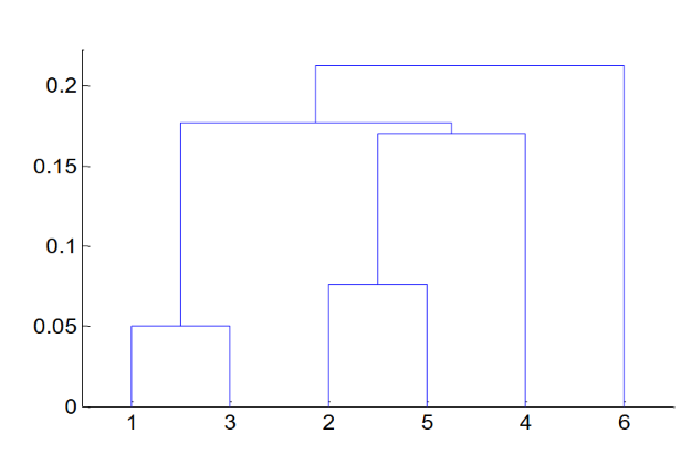
Hierarchical Cluster does not need to set the cluster number. It will generate a hierarchical tree structure called dendrogram (树状图), by cutting the dendrogram at different level, it forms clusters with different size.

There are two main types of hierarchical clustering:

• Agglomerative
• Divisive

Agglomerative is the more common method. It starts with each data point as one cluster, then repeatedly merge the closest clusters.

Divisive is the opposite. It starts with all data points in one cluster, then repeatedly split the cluster into smaller clusters.

The branch height in dendrogram represents the distance between clusters.

If two clusters are merged at lower height, they are more similar.

If two clusters are merged at higher height, they are less similar.

Different rules can be used to decide the distance between clusters, such as MIN, MAX, Group Average, and Distance Between Centroids. Different rules may produce different dendrograms and different clustering results.