3152 Lecture 9

Lecture Slide: FIT3152 Lecture 09.pdf

Previous: 3152 Lecture 8 - Ensemble Model and Artificial Neural Networks

Network

Network is a type of graph that use Vertices (nodes) to represent the entities and Edges (arcs) to represent the connections between each entities. the Network graph can use to represent many things, such as the relation between people, structure of a social network, connection between English words.

Vertices

Vertices represent the entities in the network, such as a person, computer article etc. One vertices can be connect to another vertices to represent the relationship between two vertices.

Edges

Edges is the connections between Vertices in network. It can be undirected which can represent the double way relation, or it can be directed which can represent the one way relation.

Edges may also be weighted to show the strength of the relation, can also represent cost or gain as well like what we do in Dijkstra algorithm.

Network structures

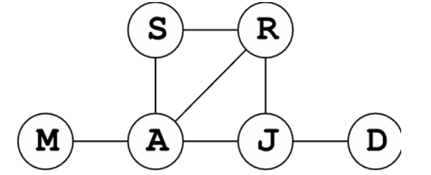
Network structure describes how vertices are connected by edges.

Term	Meaning	Example
Walk	A sequence of links, vertices can be repeated	$(M,A,J,R,J,\cdots)$
Path	A walk with no repeated vertices	$(M,A,J,R)$
Cycle	A path that begins and ends at the same vertex	$(A,S,R,A)$
Geodesic	The shortest path between two vertices	$Geodesic(R,D)=(R,J,D)$
Length	The number of links in a walk or path	$dist(M,D)=3$
Connected	There is a path between each pair of vertices	The example network is connected
Directed graph	Edges have direction, so travel is only allowed in that direction	A -> B
Loop	An edge from a vertex to itself	Edge(A,A)
Complete graph	Every vertex is joined to every other vertex	Every pair is connected
Subgraph	A subset of a graph	Graph(M,A)
Clique	A complete subgraph	Graph(A,R,J)
Simple graph	A graph with no loops or multi-edges	No repeated edge between same pair

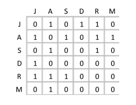
Adjacency Matrix

An adjacency Matrix can be used to represent the network by indicating the connections between individuals

Degree of vertex

Degree is the number of edges connected to a vertex, representing the size of the vertex’s neighbourhood.

For directed graphs, the degree can be separated into in-degree and out-degree.

For example, In graph above, degree(R) = 3

Network Analysis

Network analysis can describe the structure of the whole network.

Diameter

Diameter is the longest geodesic between any two vertices.

In other words, it is the longest shortest path in the network.

$$Diameter=max(dist(u,v))$$

For the network above, one longest shortest path is:

M -> A -> J -> R

So the diameter is 3.

Average Path Length

Average path length is the average geodesic distance between any two vertices in the network.

$$Average\ path\ length=\frac{\text{sum of all shortest path distances}}{\text{number of vertex pairs}}$$

For example, if the shortest path distances are:

1, 1, 2, 1, 2, 1

Then:

$$Average\ path\ length=ave(1,1,2,1,2,1)=1.333$$

Degree Distribution

Degree distribution describes how many vertices have each degree.

It describes the number of vertices by the degree that vertex has.

Degree Distribution of network:

Degree	N
0	0
1	2
2	1
3	2
4	1

Density

Density measures how many edges exist in the network compared with how many edges could possibly exist.

For an undirected simple graph:

$$den(g)=\frac{|E_g|}{|V_g|(|V_g|-1)/2}$$

Where:

$$\begin{aligned} |E_g| &= \text{number of edges in graph } g \\ |V_g| &= \text{number of vertices in graph } g \\ |V_g|(|V_g|-1)/2 &= \text{maximum possible number of edges} \end{aligned}$$

A higher density means the network is more connected.

Clustering Coefficient

Clustering coefficient is also called transitivity.

It is the proportion of triangles relative to the number of connected triples.

$$clt(g)=\frac{3\tau_{\Delta}(g)}{\tau_3(g)}$$

Where:

$$\begin{aligned} \tau_{\Delta}(g) &= \text{number of triangles in graph } g \\ \tau_3(g) &= \text{number of connected triples in graph } g \end{aligned}$$

A higher clustering coefficient means the network has more triangle-like local groups.

Vertex Importance

Vertex importance means how important or central a vertex is in the network.

The importance of a vertex can be based on:

• Number of connections with other vertices
• Centrality of vertex within the network

The number of connections can be measured by degree.

Centrality can measure the strategic power of a vertex to control information in the network.

Common centrality measures:

• Degree
• Closeness
• Betweenness
• Eigenvector

Degree Centrality

Degree centrality is based on the number of edges connected to a vertex.

A vertex with higher degree has more direct connections with other vertices.

It can be interpreted as the size of the vertex’s neighbourhood.

Closeness Centrality

Closeness centrality measures how close a vertex is to all other vertices in the network.

A vertex is close if it has small total shortest distance to all other vertices.

Closeness centrality is the inverse of the total shortest distance between one vertex and all other vertices.

$$C_{Cl}(v)=\frac{1}{\sum_{u \neq v}d(v,u)}$$

Where $d(v,u)$ is the shortest distance between vertex $v$ and vertex $u$.

For example, if the shortest distances from $J$ to all other vertices are:

1, 1, 2, 1, 2

Then:

$$C_{Cl}(J)=\frac{1}{1+1+2+1+2}=\frac{1}{7}$$

High closeness centrality means the vertex can reach other vertices with shorter paths.

So high closeness centrality means strong local influencer.

Betweenness Centrality

Betweenness centrality measures how often a vertex is between other vertices.

It counts the number of shortest paths between other vertices that pass through this vertex.

$$C_B(v)=\sum_{s\neq v\neq t}\frac{\sigma_{st}(v)}{\sigma_{st}}$$

Where:

$$\begin{aligned} C_B(v) &= \text{betweenness centrality of vertex } v \\ \sigma_{st} &= \text{the number of shortest paths from } s \text{ to } t \\ \sigma_{st}(v) &= \text{the number of shortest paths from } s \text{ to } t \text{ that pass through } v \end{aligned}$$

If there is more than one shortest path, the count may be proportional.

In the other word, betweenness centrality is the sum of the number of shortest paths between other vertices that pass through this vertex.

A vertex with high betweenness centrality can act as a bridge, hub, or relay in the network.

For example, if many shortest paths must go through vertex $J$, then $J$ has high betweenness centrality.

If a vertex is not on any shortest path between other vertices, then its betweenness centrality is 0.

Eigenvector Centrality

Eigenvector centrality measures the importance of a vertex based on the importance of its neighbours.

The idea is that connecting to important vertices makes a vertex more important.

It is difficult to calculate by hand, but the concept is useful.

For example, Google PageRank is related to this idea.

Which Centrality Measure

Different centrality measures describe different types of importance.

Degree centrality measures direct connections.

Closeness centrality measures how well a vertex is connected locally.

Betweenness centrality measures hub or bridge potential.

Eigenvector centrality measures the quality of connections.

Hand Calculation Example

For a small graph, common hand calculation questions include:

• Average path length
• Diameter
• Degree of a vertex
• Degree distribution
• Betweenness centrality
• Closeness centrality
• Cliques

Average path length is the average of all geodesic distances between pairs of vertices.

Diameter is the longest geodesic distance in the network.

Degree of a vertex is the number of edges connected to that vertex.

Clique is a subgraph where every vertex is connected to every other vertex.

For closeness centrality, first calculate the shortest distance from the chosen vertex to all other vertices, then take the inverse of the total distance.

For betweenness centrality, check which shortest paths between other vertices pass through the chosen vertex.

From the class example in slide:

• Average path length = $ave(1,1,2,1,2,1)=1.333$
• Diameter = 2
• $d_Y=3$
• Degree distribution = 3, 2, 2, 1
• $C_B(Y)=2$
• $C_{Cl}(Y)=\frac{1}{1+1+1}=0.333$
• Cliques include W-X, W-Y, X-Y, Y-Z, and W-X-Y