3152 Lecture 8

Lecture Slide: FIT3152 Lecture 08.pdf

Previous: 3152 Lecture 7 - Naive Bayes Classification and Evaluate performance Next: 3152 Lecture 9 - Networks Analysis

[!NOTE] Other Unit In FIT2086, we also mentioned this at 2086 Lecture 9 - Trees and Nearest Neighbour Methods#Random Forests

Ensemble Model

Sometimes when we work with more complex data, a single classification model like Decision Tree may not be enough. It may be too simple or unstable, so it is hard to learn many complex patterns in the data, which can lead to low accuracy or high variance. So we introduce Ensemble model.

To improve the classification model, we build a collection of ‘Experts’, which means a set of different classifier models built from the training data. These models can be trained using different samples, different attributes, or modified weights in the dataset. They can be the same type of classifier or different types of classifiers.

The result of all classifiers will be combined by methods like majority voting, sometimes with weights.

The main idea is to create a better classifier from a collection of weaker classifiers.

Ensemble model works best when:

• Individual classifiers have > 50% accuracy, which means they are better than random guessing.
• Individual classifiers are created independently, i.e. they use different data or settings etc.
• Pooling the result of each classifier will reduce the variance of the overall classification.
• Decision trees work well as the individual classifiers, we often use decision trees as the classifier model in ensemble model.

Ensemble model also has disadvantages such as longer training time, and model becomes hard to interpret compared to single model.

Bagging

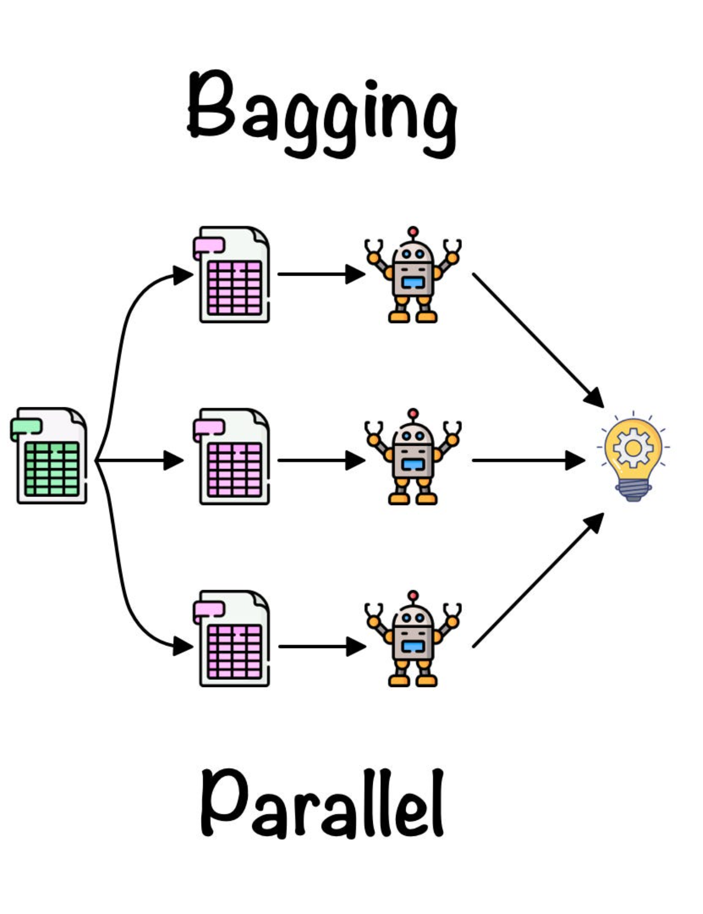
Bagging means Bootstrap Aggregation.

The main idea of Bagging is to create many different training datasets by sampling with replacement from the original training set.

Each new dataset has the same size as the original dataset, but some rows may appear multiple times and some rows may not appear.

Then we train one classifier for each dataset.

Finally, combine the classifiers by majority voting to produce the final decision.

Algorithm:

• Make multiple replicates of the original data by sampling with replacement from the training set.
• Construct a single classifier for each replicate.
• Combine the classifiers by taking a majority vote.

Bagging is useful when:

• There is noise in the data.
• The classifier is unstable, which means small changes in training data can cause large changes in the classifier.
• Examples of unstable classifiers include decision trees, neural networks and linear regression.

Bagging is not recommended for stable classifiers such as K Nearest Neighbours and Naive Bayes.

In Bagging, votes can also be translated to confidence.

For example, if we have 10 trees and 7 trees vote for class A, then the confidence for class A is:

$$\frac{7}{10}=0.7$$

Boosting

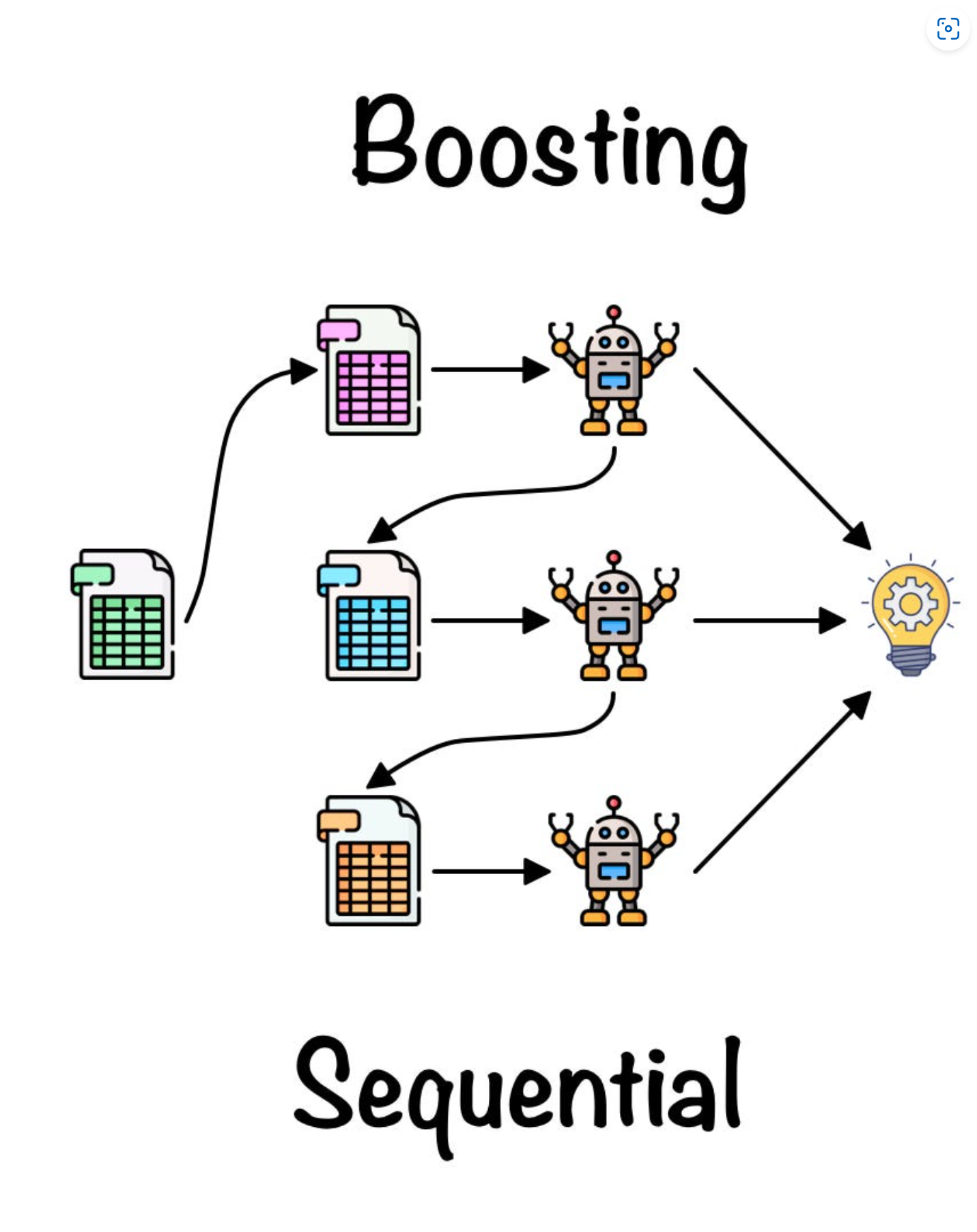
Boosting also builds multiple classifiers, but it builds them slowly by incremental improvement.

Unlike Bagging, Boosting usually uses the original dataset for all trees.

But the training examples are weighted.

At the beginning, every training example has the same weight.

After each classifier is trained, the misclassified examples will get higher weights, so the next classifier will focus more on the hard-to-classify examples.

The final classification is made by weighted sum of votes from each classifier.

More accurate classifiers have greater weight.

Algorithm:

• Assign equal weights to each point in training set, then fit a basic tree.
• Repeat n iterations.
• Update the weights of misclassified items and normalise the weights.
• Build the next tree based on the updated weights.
• Output the final classifier as weighted sum of votes from each tree.

Boosting can improve classification for imbalanced datasets, where most instances are from one class.

Boosting tends to achieve better accuracy than Bagging, but it can lead to overfitting if the number of trees is too large.

There are many Boosting algorithms, and this lecture uses Adaptive Boosting, which is AdaBoost.

Random Forest

Random Forest is a refinement of bagged decision trees.

It is specifically designed for decision trees.

The main difference between Bagging and Random Forest is:

Bagging only changes the sample data and the number of trees.

Random Forest changes the sample data, the number of trees, and also the attributes used to build each tree.

Algorithm:

• Create multiple datasets from the original training set using subsets of data points and subsets of attributes.
• Build a decision tree classifier for each dataset.
• Combine the classifiers by taking a majority vote.

Advantages of Random Forest:

• More accurate than individual trees on large datasets.
• No need to prune.
• Not sensitive to outliers.
• Overfitting is usually not a problem.

Random Forest can also output prediction confidence.

For example, if many trees vote for one class, the model will have higher confidence for that class.

Compare

Metrics\Model	Bagging	Boosting	Random Forest
Basic idea	Train many classifiers on bootstrap samples	Train classifiers step by step, focus more on previous mistakes	Train many decision trees using subsets of rows and attributes
Data used	Resampled data with replacement	Original data, but examples have different weights	Resampled data and subset of attributes
Combination method	Majority voting	Weighted voting	Majority voting
Good for	Noisy data and unstable classifiers	Imbalanced data and improving accuracy	Large datasets and decision tree based classification
Main risk	Not useful for stable classifiers	Can overfit if too many trees	Hard to interpret
Base classifier	Often decision tree	Often decision tree	Decision tree

Cross Validation

All these models can be further improved by cross validation.

Cross validation helps test model performance on different train/test splits.

This can help us understand which parameter settings affect model performance.

Artificial Neural Network (ANN)

Artificial Neural Networks are computer models inspired by neural behaviour in the human brain.

ANNs can be used for many different problems, such as prediction, classification, pattern recognition and optimisation.

The main idea is that ANN can “learn” by adjusting the weight of each connection between neurons.

ANNs are usually accurate, and can handle redundant attributes and noisy data.

Large ANNs give rise to deep learning.

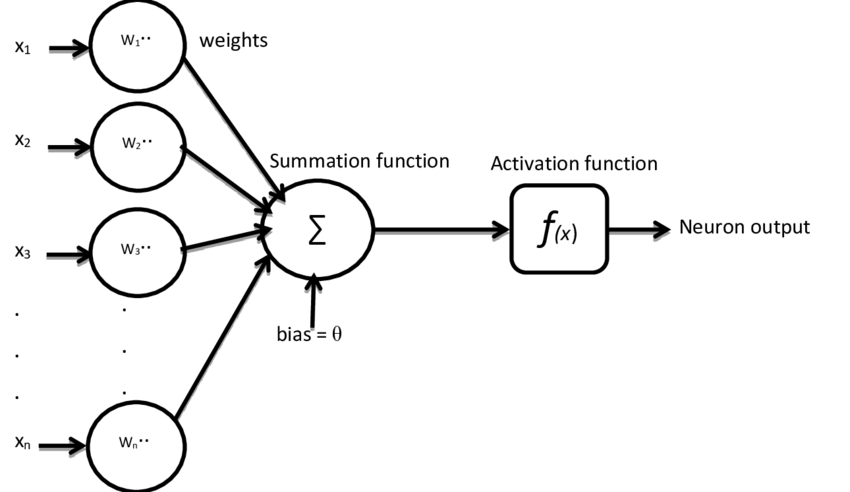
Artificial Neuron

An artificial neuron receives several input values.

Each input has a weight.

The neuron calculates the weighted sum of inputs, then subtracts a bias or threshold.

Then the result is passed into an activation function to produce the output.

The basic form is:

$$y=g(w_1x_1+w_2x_2+\cdots+w_nx_n-\theta)$$

Where:

$$\begin{aligned} x_i &= \text{input variable } i \\ w_i &= \text{weight for input } i \\ \theta &= \text{threshold / bias} \\ g(.) &= \text{activation function} \\ y &= \text{output} \end{aligned}$$

So the operation of artificial neuron is:

• Input is given by variables $x_1,x_2,\cdots,x_n$.
• Each input is multiplied by its weight.
• The neuron calculates the weighted sum.
• Bias or threshold is subtracted.
• Activation function converts the activation potential into output.

Activation Function 激活函数

Activation function decides how the neuron output should be produced from the activation potential.

It also limits the output of the neuron.

Common activation functions include:

• Step function
• Ramp function
• Logistic function
• Hyperbolic Tangent, Tanh
• Gaussian function

Fully differentiable activation functions are useful because they allow the model to optimise weights during training.

Network Architecture

The structure of ANN determines:

• The number of inputs the model can accept.
• The number of outputs the model can produce.
• The complexity of interactions that can be modelled.

There are usually three types of layers:

• Input layer
• Hidden layer
• Output layer

Input layer receives the input variables.

Hidden layers learn the relationship and interaction between input variables.

Output layer produces the final prediction or classification.

Single Layer Feedforward ANN

Single layer feedforward ANN has n inputs and m outputs.

Information only flows in one direction, from input to output.

There is no feedback loop.

Multiple Layer Feedforward ANN

Multiple layer feedforward ANN has one or more hidden layers between input and output.

Hidden layers allow mixing and interaction between neurons.

This helps the neural network solve complex and non-linear problems.

Examples include:

• Optimisation
• Pattern recognition
• Classification

More hidden layers can model more complex interactions.

TODO: Add MLP

Recurrent / Feedback Architecture

In recurrent or feedback architecture, outputs of neurons can become inputs for earlier layers.

This allows dynamic information processing.

It is useful for time-varying systems, such as:

• Time series prediction
• Optimisation
• Process control

Training ANN

Training ANN means adjusting the weights of each connection and the thresholds of neurons.

The goal is to make the predicted output close to the actual output in the training set.

For supervised learning, training is an iterative optimisation process.

It tries to reduce the error between known output and predicted output.

For unsupervised learning, the goal is more about producing clusters of similar subsets of the data.

Setting Up ANN

Before training ANN, the data needs pre-processing.

Important requirements:

• One input neuron for each input variable.
• One output neuron for each output class.
• Inputs should be numerical.
• Data should be normalised.
• Categorical data needs to be converted into binary columns using one hot encoding.
• There should be no missing values.

For classification with multiple classes, we need multiple output nodes.

For example, Iris dataset has 3 classes, so it needs 3 output nodes:

• setosa
• versicolor
• virginica

Each class can be represented by an indicator variable.