3152 Lecture 7

Lecture Slide: FIT3152 Lecture 07.pdf

Previous: 3152 Lecture 6 - Decision Tree Next: 3152 Lecture 8 - Ensemble Model and Artificial Neural Networks

Naive Bayes Assumption

Assumption:

The attributes are conditionally independent given the classifier.

This means that once we know the class $C$, each attribute $A_i$ does not depend on the other attributes.

Also assume the attributes are independent with each other, so the joint probability in the denominator can be rewritten as a multiplication of each attribute probability.

$$\begin{aligned} A_i &= \text{attribute } i \\ C &= \text{classifier / class label} \\ \\ P(A_i) &= \text{probability of attribute } A_i \\ P(C) &= \text{prior probability of class } C \\ P(A_i \mid C) &= \text{probability of attribute } A_i \text{ given class } C \\ P(C \mid A_i) &= \text{probability of class } C \text{ given attribute } A_i \end{aligned}$$

Bayes’ Theorem

$$P(C \mid A) = \frac{P(C)P(A \mid C)}{P(A)}$$

For multiple attributes:

$$P(C \mid A_1 \cap A_2 \cap A_3 \cap \cdots \cap A_n) = \frac{ P(C)P(A_1 \cap A_2 \cap A_3 \cap \cdots \cap A_n \mid C) }{ P(A_1 \cap A_2 \cap A_3 \cap \cdots \cap A_n) }$$

Since the attributes are conditionally independent given $C$:

$$P(A_1 \cap A_2 \cap A_3 \cap \cdots \cap A_n \mid C) = P(A_1 \mid C)P(A_2 \mid C)P(A_3 \mid C)\cdots P(A_n \mid C)$$

Since the attributes are also assumed to be independent with each other:

$$P(A_1 \cap A_2 \cap A_3 \cap \cdots \cap A_n) = P(A_1)P(A_2)P(A_3)\cdots P(A_n)$$

Therefore:

$$P(C \mid A_1 \cap A_2 \cap A_3 \cap \cdots \cap A_n) = \frac{ P(C)P(A_1 \mid C)P(A_2 \mid C)P(A_3 \mid C)\cdots P(A_n \mid C) }{ P(A_1)P(A_2)P(A_3)\cdots P(A_n) }$$

Evaluate Classifier Performance

[!NOTE] Recap Also in FIT2086: 2086 Lecture 7 - Classification and Logistic Regression#Evaluating Classifiers

Confusion Matrix

Confusion Matrix is a summary of the test results.

	Predicted Class = Yes	Predicted Class = No
Actual Class = Yes	TP	FN
Actual Class = No	FP	TN

TP means the actual class is positive, and the model also predicts positive.

FN means the actual class is positive, but the model predicts negative.

FP means the actual class is negative, but the model predicts positive.

TN means the actual class is negative, and the model also predicts negative.

Measurements:

Accuracy 在所有数据里，有多少被正确识别了，不论是N还是P:

$$Accuracy=\frac{TP+TN}{TP+TN+FP+FN}$$

Precision 有多少预测的Positive是真的Positive:

$$Precision=\frac{TP}{TP+FP}$$

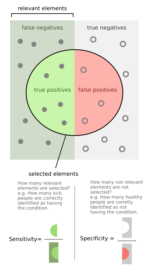
Recall, Sensitivity (True Positive Rate) 有多少Actural Positive被识别为了Positive:

$$Recall=TPR=\frac{TP}{TP+FN}$$

Specificity (True Negative Rate) 有多少Actural Negative被识别为了Negative:

$$TNR=\frac{TN}{TN+FP}$$

FPR(False Positive Rate) 有多少Actural Negative被误报为了Positive:

$$FPR=\frac{FP}{TN+FP}$$

F1-Score:

$$F1=2\times\frac{Precision\times Recall}{Precision+Recall}$$

F1-Score is the harmonic mean of precision and recall. It is useful for imbalanced datasets.

ROC

ROC curve is plotting the TPR (Sensitivity) on y axis against FPR (False Positive Rate = 1-Specificity) on x axis.

One classifier will present as a single point on the ROC curve, and by changing the threshold of the classifier, it forms another new point, and forms a curve.

TPR indicates how good the classifier is for correctly predicting yes when it should predict yes.

FPR is also called false alarm rate.

Changing the confidence threshold changes the predicted class, so TP, FP, TN, FN will also change.

Then we can calculate a new TPR and FPR for each threshold, and plot all the points to get the ROC curve.

Some important points:

$(0,0)$ means declare everything to be negative class.

$(1,1)$ means declare everything to be positive class.

$(0,1)$ is the ideal point, where TPR is 1 and FPR is 0.

The diagonal line means random guessing.

A curve below the diagonal line means the prediction is worse than guessing.

AUC

Area Under Curve, basically measuring the area under ROC curve, the larger the AUC, the better the model can separate

the positive class and negative class.

AUC is a single value for measuring the overall performance of the classifier.

The value is between 0 and 1.

AUC = 0.5 means random guessing.

AUC = 1 means perfect classifier.

For a realistic classifier, AUC should not be less than 0.5.

It can also be understood as the probability that the classifier ranks a randomly chosen positive instance higher than a randomly chosen negative instance.

Lift

Lift is another way to evaluate binary classification or prediction model.

It measures the improvement from using the model compared with not using the model.

$$Lift=\frac{\text{success rate with model}}{\text{success rate without model}}$$

If the model outputs probability or confidence, we can sort the instances by predicted confidence from high to low.

Then select the top sample, and compare its success rate with the success rate of the whole dataset.

For example, if there are 150 instances and 50 are positive:

$$\text{success rate without model}=\frac{50}{150}=33.33\%$$

If we select the top 10 instances by model confidence, and 7 of them are positive:

$$\text{success rate with model}=\frac{7}{10}=70\%$$

Then:

$$Lift=\frac{7/10}{50/150}=2.1$$

This means using the model gives 2.1 times higher success rate than selecting randomly.